ANOVA3Way
Advanced Analysis Library Only
AnalysisLibErrType ANOVA3Way (double observationsArray[], ssize_t levelAArray[], ssize_t levelBArray[], ssize_t levelCArray[], ssize_t totalObservations, ssize_t cellCount, ssize_t levelsInA, ssize_t levelsInB, ssize_t levelsInC, double information[4][8], double *significanceA, double *significanceB, double *significanceC, double *significanceAB, double *significanceAC, double *significanceBC, double *significanceABC);
Purpose
Takes an array of experimental observations made at various levels of three factors and performs a three-way analysis of variance in any of the following models:
- Model 1—Fixed effects with interaction and L > 1 observations per cell.
- Model 2—Any of the six mixed-effects models, where one or two factors are taken to have fixed effects but the remaining factors are taken to have random effects, with interaction and L > 1 observations per cell.
- Model 3—Random effects with interaction and L > 1 observations per cell.
Any ANOVA looks for evidence that the factors, or interactions among the factors, have a significant effect on experimental outcomes. The method for finding significance varies among models.
| For the following sections, let | observationsArray = y |
| levelA_Array = levelA | |
| levelB_Array = levelB | |
| levelC_Array = levelC | |
| totalObservations = N | |
| cellCount = L | |
| levelsInA = a | |
| levelsInB = b | |
| levelsInC = c | |
| significanceA = sigA | |
| significanceB = sigB | |
| significanceC = sigC | |
| significanceAB = sigAB | |
| significanceAC = sigAC | |
| significanceBC = sigBC | |
| significanceABC = sigABC |
Factors, Levels, and Cells
A factor is a way of categorizing data. You can categorize data into levels, beginning with level 0. For example, if you perform a measurement on individuals, such as counting the number of sit-ups they can perform, one such categorization method is age. For age, you might have three levels, as shown in the following table.
| Level | Age |
|---|---|
| 0 | 6 years to 10 years |
| 1 | 11 years to 15 years |
| 2 | 16 years to 20 years |
Another possible factor is eye color, with the levels shown in the following table.
| Level | Eye Color |
|---|---|
| 0 | blue |
| 1 | brown |
| 2 | green |
| 3 | hazel |
A third factor might be height with levels in blocks of 10 cm. A cell of data consists of all those experimental observations that fall in particular levels of the three factors. In this instance, a cell might consist of those observations made on hazel-eyed individuals between 11 years old and 15 years old who are between 151 cm and 160 cm tall. The number of observations that fall in each cell must be a constant number L that does not vary between cells.
Random and Fixed Effects
A factor is taken as a random effect when the factor has a large population of levels you want to draw conclusions about, but that you cannot sample at all levels. Levels are sampled at random in the hope of generalizing about all levels.
A factor is taken as a fixed effect when the factor can be sampled from all levels you want to draw conclusions about.
The input parameters a, b, and c represent the number of levels in factors A, B, and C, respectively. If factor A is random, set a to a negative value. In the same way, set b and c to negative values if B and C are random.
General Method
Each of the previous models breaks up the total sum of squares (tss), which is a measure of the total variation of the data from the overall population mean, into a number of component sums of squares, so that:
tss = ssa + ssb + ssc + ssab + ssac + ssbc + ssabc + sse
Each component in the sum is a measure of variation attributed to a certain factor or interaction among the factors. In this instance, ssa is a measure of the variation as a result of factor A; ssb is a measure of the variation as a result of factor B; ssc is a measure of the variation as a result of factor C; ssab is a measure of the variation as a result of the interaction between factors A and B; and so on for ssac, ssbc, and ssabc. The variable sse is a measure of the variation as a result of random fluctuation.
If factor A has a strong effect on the experimental observations, msa is relatively large. You can look at specific ratios of these averages because you know how they are statistically distributed. You can therefore determine how likely it is that factor A is as relatively large as it is.
Statistical Model
Let yp, q, r, s be the sth observation at the pth, qth, and rth levels of A, B, and C, respectively, where s = 0, 1, . . ., L – 1.
Express each observation as the sum of eight components so that
yp, q, r, s = μ + αp + βq + γr + (αβ)p, q + (αγ)p, r + (βγ)q, r + (αβγ)p, q, r + εp, q, r, s
| where | μ represents a standard effect present in each observation |
| αp, βq, and γr are the effects of factors A, B, and C respectively | |
| (αβ)p, q, (αγ)p, r, (βγ)q, r, and (αβγ)p, q, r are the effects of the corresponding interactions | |
| εp, q, r, s is a random fluctuation |
Assumptions
- Assume that for each p, q, r, and s, εp, q, r, s is normally distributed with mean 0 and variance σ2ε.
- If a factor such as A is fixed, assume that the populations of measurements at each level are normally distributed with mean αp and variance σ2A. All the populations at each of the levels have the same variance. In addition, assume that all the αp means sum to zero. Make analogous assumptions for B and C.
- If a factor such as A is random, assume that the effect of the level of A itself, αp, is a random variable normally distributed with mean 0 and variance σ2A. Make analogous assumptions for B and C.
- If all the factors, such as A and B, associated with the effect of an interaction (αβ)p, q are fixed, assume that the populations of measurements at each level are normally distributed with mean (αβ)p, q and variance σ2AB. For any fixed p, the (αβ)p, q means sum to zero when summing over all q. Similarly, for any fixed q, the (αβ)p, q means sum to zero when summing over all p.
- If any of the factors, such as A and B, associated with the effect of an interaction (αβ)p, q are random, assume that the effect is a random variable normally distributed with mean 0 and variance σ2AB. If A is fixed but B is random, assume also that for any fixed q, the (αβ)p, q means sum to zero when summing over all p. Similarly, if B is fixed but A is random, assume also that for any fixed p, the (αβ)p, q means sum to zero when summing over all q.
- Assume that all effects taken to random variables are independent.
Hypotheses
Each of the following hypotheses are different ways of stating that a factor or an interaction among factors has no effect on experimental outcomes. Start by assuming that there are no effects and then seek evidence to contradict these assumptions. The seven hypotheses are as follows:
- For hypothesis A, αp = 0 for all levels of p if factor A is fixed; σ2A = 0 if factor A is random.
- For hypothesis B, βq = 0 for all levels of q if factor B is fixed; σ2B = 0 if factor B is random.
- For hypothesis C, γr = 0 for all levels of r if factor C is fixed; σ2C = 0 if factor C is random.
- For hypothesis AB, (αβ)p, q = 0 for all levels of p and q if factors A and B are fixed; σ2AB = 0 if either factor A or B is random.
- For hypothesis AC, (αγ)p, r = 0 for all levels of p and r if factors A and C are fixed; σ2AC if either factor A or C is random.
- For hypothesis BC, (βγ)q, r = 0 for all levels of q and r if factors B and C are fixed; σ2BC if either factor B or C is random.
- For hypothesis ABC, (αβγ)p, q, r = 0 for all levels of p, q, and r if factors A, B, and C are fixed; σ2ABC if any of the factors A, B, or C are random.
Testing the Hypotheses
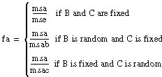
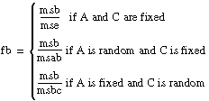
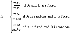
For each hypothesis, ANOVA3Way generates a number so that if the hypothesis is true, that number is from a particular F-distribution.
For example, in the fixed-effects model, the number fa = msa/mse, associated with hypothesis A, is from an F-distribution with a – 1 and abc(L – 1) degrees of freedom, given that hypothesis A is true. ANOVA3Way calculates the probability that a number taken from a particular F-distribution is larger than the F-value. For example,
sigA = prob(X > fa) where X is from F (a – 1, abc(L – 1))
Use the probabilities sigA, sigB, sigC, sigAB, sigAC, sigBC, and sigABC to determine when to reject the associated hypotheses A, B, C, AB, AC, BC, and ABC by choosing a level of significance for each hypothesis. The level of significance determines how likely you are to reject the hypothesis when it is in fact true. Thus, the level of significance should be small, for example, 0.05. Remember that the smaller the level of significance, the less likely you are to reject the hypothesis.
Reject a particular hypothesis when the associated output parameter sigA, sigB, sigC, sigAB, sigAC, sigBC, or sigABC is less than the level of significance you choose for that hypothesis. If A is a random effect, the chosen level of significance is 0.05, and sigA = 0.03, you must reject the hypothesis that σ2A = 0 and conclude that factor A has an effect on the experimental observations.
With some models, no appropriate tests exist for certain hypotheses. In these cases, ANOVA3Way sets the output parameters directly involved with the testing of those hypotheses to –1.0.
Formulas
Let yp, q, r, s be the sth observation at the pth, qth, and rth levels of A, B, and C, respectively, where s = 0, 1, . . ., L – 1.
Let
aa = |a|
bb = |b|
cc = |c|


T = the total sum of all observations:


Then
ssa = A – CF

ssb = B – CF

ssc = C – CF

ssab = AB – A – B + CF

ssac = AC – A – C + CF

ssbc = BC – B – C + CF

ssabc = S – AB – AC – BC + A + B + C – CF


If 


assume that f is from an F-distribution with dof1 and dof2 degrees of freedom.
Example Scenario
Suppose that researchers want to know how the number of hours of sunlight, the amount of rainfall, and the average temperature affect the yield of a crop. Each factor, sunlight, rainfall, and temperature, is divided into three levels as shown in the following tables of sunlight, rainfall, and temperature levels.
| Level | Sunlight (Factor A) |
|---|---|
| 0 | 5 hours |
| 1 | 6 hours |
| 2 | 7 hours |
| Level | Rainfall (Factor B) |
|---|---|
| 0 | 2 inches |
| 1 | 3 inches |
| 2 | 4 inches |
| Level | Temperature (Factor C) |
|---|---|
| 0 | 76 – 80 degrees |
| 1 | 81 – 85 degrees |
| 2 | 86 – 90 degrees |
A particular plot planted with the crop might appear in any one of the 27 different combinations of these levels with the three factors. For example, one combination might be 6 hours of sunlight with 2 inches of rainfall and an average temperature between 76 degrees and 80 degrees, recorded as (1,0,0). Call these combinations cells.
The researchers set up 54 plots in various geographical locations chosen so that two plots fall in each of the 27 cells. To measure the productivity of a particular plot, they record the crop production. Let sunlight be factor A, rainfall be factor B, and temperature be factor C.
The following table shows their results.
| (A, B, C) | Bushels produced from each plot |
|---|---|
| (0, 0, 0) | 128 122 |
| (0, 0, 1) | 113 108 |
| (0, 0, 2) | 116 116 |
| (0, 1, 0) | 132 129 |
| (0, 1, 1) | 119 121 |
| (0, 1, 2) | 126 113 |
| (0, 2, 0) | 118 114 |
| (0, 2, 1) | 141 133 |
| (0, 2, 2) | 121 123 |
| (1, 0, 0) | 119 118 |
| (1, 0, 1) | 111 115 |
| (1, 0, 2) | 143 140 |
| (1, 1, 0) | 127 129 |
| (1, 2, 2) | 112 113 |
| (1, 1, 1) | 128 120 |
| (1, 1, 2) | 122 121 |
| (1, 2, 0) | 114 115 |
| (1, 2, 1) | 116 113 |
| (2, 0, 0) | 135 131 |
| (2, 0, 1) | 145 145 |
| (2, 0, 2) | 152 147 |
| (2, 1, 0) | 137 141 |
| (2, 1, 1) | 171 171 |
| (2, 1, 2) | 135 131 |
| (2, 2, 0) | 143 144 |
| (2, 2, 1) | 145 147 |
| (2, 2, 2) | 121 123 |
To perform a three-way analysis of variance in the fixed-effect model using ANOVA3Way, you store all the numbers of bushels in a double-precision array y of size 54. The integer arrays levelA, levelB, and levelC record the cells in which observations were made. For any particular i, you set these arrays such that yi is the number of bushels a plot produces in the (levelAi, levelBi, levelCi) cell. For example,
(levelAi, levelBi, levelCi) = (0, 1, 1)
yi = 119 or 121
are valid combinations. Therefore, you can set up the input arrays y, levelA, levelB, and levelC in this example for ANOVA3Way as follows:
y = 128, 122, 113, 108, 116, 116, 132, 129, . . .
levelA = 0, 0, 0, 0, 0, 0, 0, 0, . . .
levelB = 0, 0, 0, 0, 0, 0, 1, 1, . . .
levelC = 0, 0, 1, 1, 2, 2, 0, 0, . . .
Running the code in the following example produces:
sigA = 1.11e–16
sigB = 1.3e–8
sigC = 0.0072
sigAB = 1.2e–8
sigAC = 2.0e–4
sigBC = 4.5e–10
sigABC = 4.8e–10
For a level of significance such as 0.05, the ANOVA3Way results show that the researchers must reject the hypotheses that sunlight, rainfall, and temperature have no effect on the crop yield. In other words, all three factors have a significant effect on crop yield.
Example Code
double y[54], sigA, sigB, sigC, sigAB, sigAC, sigBC, sigABC, info[8][4];
int levelA[54], levelB[54], levelC[54];
int L, a, b, c;
int status;
L = 2; /* two observations per cell */
a = 3; /* three levels for factor A, Sunlight */
b = 3; /* three levels for factor B, Rainfall */
c = 3; /* three levels for factor C, Temperature */
/* Read in recorded data y[54], levelA[54], levelB[54], and levelC[54]. */
status = ANOVA3Way(y, levelA, levelB, levelC, 54, L, a, b, c, info,
&sigA, &sigB, &sigC, &sigAB, &sigAC, &sigBC, &sigABC);
Parameters
| Input | ||
| Name | Type | Description |
| observationsArray | double [] | Array of experimental observations. The number of elements in observationsArray should total cellCount × levelsInA × levelsInB × levelsInC. |
| levelAArray | ssize_t [] | The ith element tells in what level of factor A the ith observation falls. The number of values in levelA_Array should total cellCount × levelsInA × levelsInB × levelsInC. |
| levelBArray | ssize_t [] | The ith element tells in what level of factor B the ith observation falls. The number of values in levelB_Array should total cellCount × levelsInA × levelsInB × levelsInC. |
| levelCArray | ssize_t [] | The ith element tells in what level of factor C the ith observation falls. The number of values in levelC_Array should total cellCount × levelsInA × levelsInB × levelsInC. |
| totalObservations | ssize_t | Total number of experimental observations. The number of values in totalObservations should total cellCount × levelsInA × levelsInB × levelsInC. |
| cellCount | ssize_t | Number of observations per cell. Observations made at particular levels x, y, and z of A, B, and C respectively, are said to fall in the (x,y,z) cell. cellCount is the number of observations recorded at those levels of A, B and C. ANOVA3Way handles balanced data in which all cells have the same cell count. cellCount > 1 |
| levelsInA | ssize_t | Number of levels in factor A. If factor A is a fixed effect, (levelsInA) > 1. If factor A is a random effect, (levelsInA) < –1. |
| levelsInB | ssize_t | Number of levels in factor B. If factor B is a fixed effect, (levelsInB) > 1. If factor B is a random effect, (levelsInB) < –1. |
| levelsInC | ssize_t | Number of levels in factor C. If factor C is a fixed effect, (levelsInC) > 1. If factor C is a random effect, (levelsInC) < –1. |
| Output | ||
| Name | Type | Description |
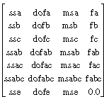
| information | double [][4] | A 4-by-8 matrix as follows:
where ss designates sums of squares, dof designates degrees of freedom of ss, ms designates mean squares, and f designates F-distributions, depending on the statistical model. Column 0 holds the 8 sums of squares due to a, b, c, ab interaction, ac interaction, bc interaction, abc interaction, and random fluctuation. Column 1 holds the degrees of freedom of the respective sums of squares. Column 2 contains the 8 corresponding mean squares. Column 3 contains the 7 corresponding F-values and a 0.0. F-values are set to –1.0 if no appropriate F-test exists. |
| significanceA | double | Level of significance at which you must reject hypothesis A. |
| significanceB | double | Level of significance at which you must reject hypothesis B. |
| significanceC | double | Level of significance at which you must reject hypothesis C. |
| significanceAB | double | Level of significance at which you must reject hypothesis AB. |
| significanceAC | double | Level of significance at which you must reject hypothesis AC. |
| significanceBC | double | Level of significance at which you must reject hypothesis BC. |
| significanceABC | double | Level of significance at which you must reject hypothesis ABC. |
Return Value
| Name | Type | Description |
| status | AnalysisLibErrType | A value that specifies the type of error that occurred. Refer to analysis.h for definitions of these constants. |
Additional Information
Library: Advanced Analysis Library
Include file: analysis.h
LabWindows/CVI compatibility: LabWindows/CVI 3.1 and later